CS-433 (Machine Learning)
1. Linear Regression
, where is the feature vector with a 1 in front (adding a constant) and the weight vector for predicting label
2. Loss functions
Desirable: symmetric around 0, penalise large and very large mistakes similarly
- → not good for outliers
- → good for outliers
Convexity
Function is convex if for any and for any we have:
A strictly convex function has a unique global minimum. For convex functions, every local minimum is a global minimum. Sums of convex functions and compositions of convex functions with convex non-decreasing functions are convex.
3. Optimisation
Find such that it is
Grid search: parameters per dimension → evaluations and no guarantee to find minimum
Gradient descent:
-
- Linear MSE:
-
-
- Global complexity
SGD:
-
- Cheap but unbiased estimate of the gradient
- Global complexity
Mini-batch SGD:
- , B is a subset of the N samples
-
Subgradient descent:
- Convexity for differentiable functions:
- Subgradient :
Projected gradient descent:
- Intersections of convex sets are convex
- Projection on convex constraint set after each gradient descent step
- Turn into unconstrained problem: penalty function if not in
4. Least squares
Gram matrix . Closed form for optimal given by . The Gram matrix is invertible iff has full column rank. Complexity is
- -regularisation closed form with :
- Eigenvalues of are at least
5. Maximum Likelihood
Maximising the likelihood instead of minimising the loss. Our data is , where is a random variable (e.g. Gaussian) that is iid across .
Log likelihood
6. Regularisation
Penalise complex models:
- -regularisation (ridge):
- Gradient is
- Model small in magnitude
- -regularisation (lasso):
- Gradient is
- Model is sparse
- -regularisation (lasso):
- Shrinkage, dropout, weight decay, early stopping
7. Generalisation, model selection and validation
Generalisation gap: how far is the test from the true error?
Given different models , an iid test set (that follows the true data distribution) and a loss :
To remove the absolute value, put 2 in front of the square root and take the values of for which the functions and have the smallest empirical or true risk respectively.
Hoeffding inequality , are the loss functions
Hoeffding lemma , and RV with
K-fold cross validation returns an unbiased estimate of the generalisation-error and its variance
8. Bias-variance decomposition
Bias and variance of the prediction considering that the input sample is a random variable
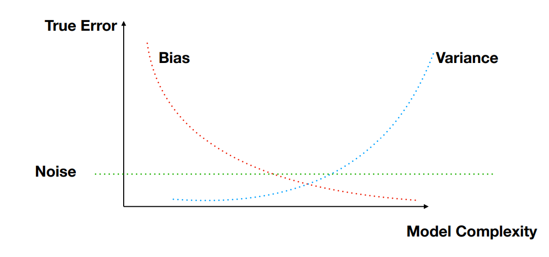
Noise → Strict lower bound, as independently random and impossible to predict (1st term)
Bias → how far off in general the model’s predictions are from the correct value (2nd term)
Variance → How much the predictions for a given point vary between realisations of the training set (3rd term)
9. Classification
The optimal classification performance is the Bayers classifier
Loss functions
- (0-1 Loss) → which is 1 if and 0 if
- True risk for classification for a predictor →
- Convex and continuous losses (:
- quadratic loss → symmetric but only works for
- hinge loss → penalty on (prediction wrong or not confident)
- logistic loss → always penalising
Non-parametric
Approximate conditional distribution via local averaging (KNN)
Parametric
Approximate true distribution via training data → minimise empirical risk (ERM)
Instead of learning function , we learn a continuous function and predict with . We replace the 0-1 loss by a convex and continuous surrogate :
In the over-parameterisation regime, the training data is well fit with a regressor → a good regressor can be used as a classifier
10. Logistic regression
Logistic function . We have and
Robust against outliers and unbalanced data. If , then for
Optimality:
- linear for :
- generic for :
- generic for :
Gradient:
- linear problem convex and
Hessian:
- , where
- Hessian is psd → loss is convex
- Newton’s method:
When data is linearly separable, weights even though all points are well separated. Solution: add regularisation
11. Support vector machines (SVM)
We consider . Margin of a hyperplane
Hard SVM - 3 equivalent formulations
- such that
- such that
- such that →
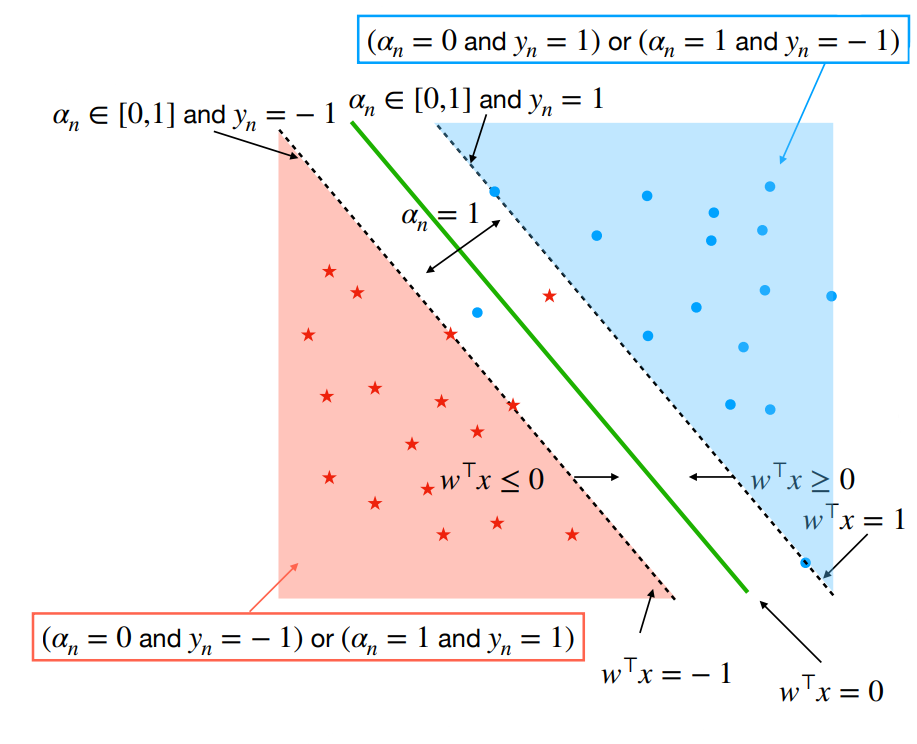
Soft SVM - non linearly separable data
Maximise margin while allowing some constraints to be violated
. Continuous but non-smooth → subgradients
Dual formulation
Define a function such that . is convex in and concave in .
Primal problem:
Dual problem:
where and . is psd and only depends on kernel matrix.
- if is on the right side, outside of the margin (
- if is on the right side and on the margin (
- if is on the inside the margin or on the wrong side (
- Points for which are called support vectors (model only depends on support vectors)
12. Nearest Neighbour Classifiers
KNN can be used for:
- regression: for point , find the closest points (the points in the neighbourhood) → the estimate is then given by
- classification: get closest neighbours of and count how many are in groups or → assign group of point depending on the majority group in the neighbourhood
Small → complex decision boundary → low bias, high variance (overfitting)
Large → when prediction is constant → high bias, low variance
Curse of dimensionality: i.i.d. points uniform in
Generalisation bound for 1-NN:
- Bayes classifier minimises over all classifiers where
- Bayes risk:
- Assumption: , : (Lipschitz with ct. c)
→ nearby points are likely to share the same label
- Claim:
- To achieve constant error we need
-
- Let , then sample has probability to have a neighbour in in the box at distance ( is Box edge lenght) and probability to not have a neighbour in the box (closest neighbour )
-
- Local averaging methods aim to approximate the Bayes’ predictor directly by approximating the conditional distribution . For , 1-NN is competitive with Bayes’ classifier
13. Kernel trick
Covariance matrix , Kernel matrix
→ Ridge regression complexity
Representer theorem: For any loss there exists , where is any increasing regularisation term, such that
Kernel trick: Kernel function → computation of linear classifiers in high-dimensional space without computing directly in that space. Prediction with kernel: (non-linear prediction in space but linear in feature space )
- Linear kernel:
- Quadratic kernel: (for )
- Polynomial kernel:
(for )
- Radial basis function (RBF) kernel:
- :
- : for
Building new kernels from existing ones:
- is a kernel for
- is a kernel
Mercer’s condition: such that iff
- kernel function is symmetric:
- kernel matrix is psd:
14. Neural Networks
Learn non-linear function to transform into a good feature representation for predictions.
Multi-layer perceptron (MLP) structure
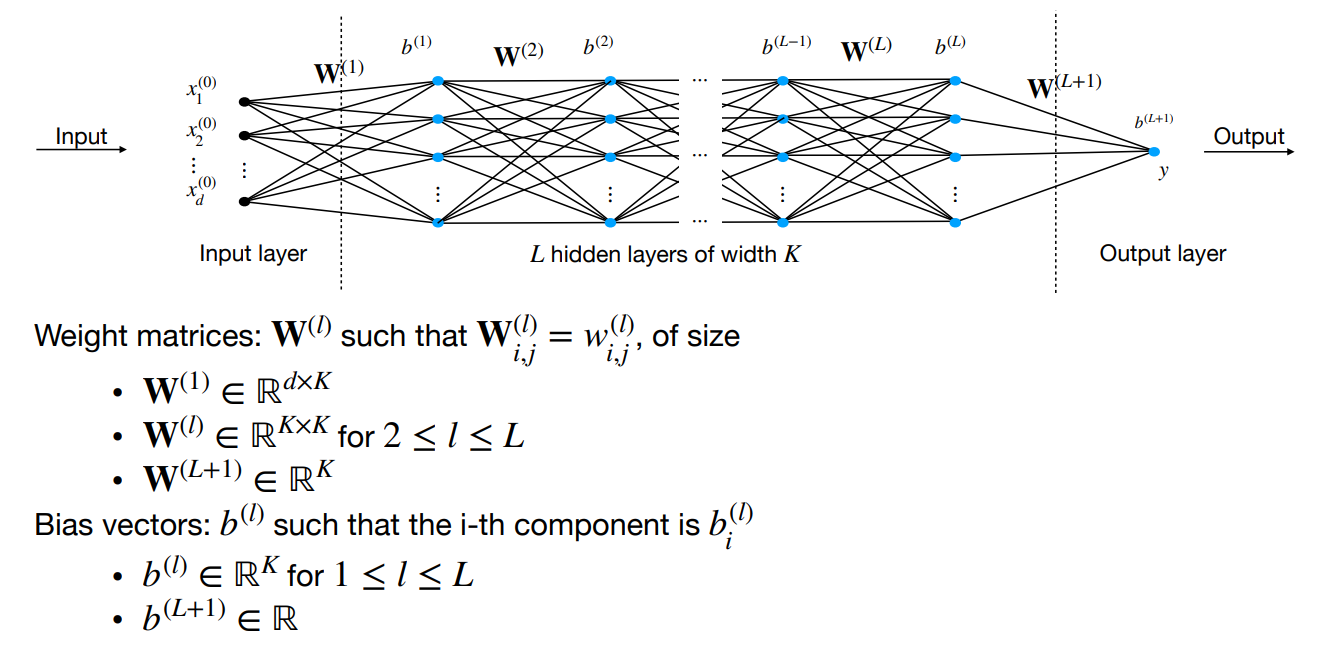
Network with hidden layers with neurons each. The output of hidden layer is
, where the weights and biases are learnable → learnable parameters. The global function is the composition
- Inference:
- Regression →
- Binary classification with →
- Multi-Class classification →
- Training
- Regression →
- Binary classification with →
- Multi-Class classification →
- Activation functions:
sigmoid
, ReLU , GeLU
Representation power
- All sufficiently smooth function can be approximated by a one-hidden-layer NN ( norm):
, → the smaller, the smoother
- A NN with sigmoid activation and at most two hidden layers can approximate well a smooth function in -norm
- Approximate the function integral in the Riemann sense by a sum of rectangles
- Represent each rectangle using two nodes in the hidden layer of a neural network
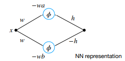
- Compute the sum of all nodes in the hidden layer (considering appropriate weights and signs) to get the final output → NN with one hidden layer containing nodes for a
Riemann sum with
rectangles
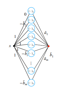
- approximation result: continuous on . , it exists piecewise linear (pwl) continuous such that
- pwl can be written as combination of ReLU
- can be implemented as a one-hidden-layer NN with ReLU activation
Training (SGD) - Backpropagation
Searching using SGD→ non-convex
Forward pass:
-
-
-
Backward pass:
-
-
Derivatives:
-
-
Parameter initialisation: vanishing/exploding gradient → He initialisation. For ReLU networks, initialise weights as
Normalisation layers: dynamically stabilise training process → faster convergence
- Batch normalisation: ( for numerical stability)
Learnable parameters to reverse normalisation:
Prediction should not depend on batch → estimate and and use for inference. Requires sufficiently large batches for good approximations
- Layer normalisation: Same but summing over to get and
Batch independent → use same normalisation for training and inference
Convolutional nets
Image size . Convolution where is a local filter with learnable weights. only depends on values of close to → sparsely connected
- Padding: for borders, use zero padding or valid padding (reduces dimensionality)
- Multiple channels: possible to use channels (filters) on one input
- Pooling: down-sampling
- max pooling: returns max value of feature portion covered by kernel
- average pooling: returns average value of feature portion covered by kernel
- Hyperparameters: pooling/convolution size/type/stride. Generally: and
- Weight sharing: back-propagation ignoring weights are shared and summing gradients of edges sharing weights
Regularisation
Residual networks: skip connections around some layers : lower training loss
Data augmentation: generate new data with same labels by corrupting existing data → robust
Weight decay: regularise weights without regularising biases. No direct regularisation effect (scale invariance) but training dynamics differ
Dropout: at each training step, retain nodes in layer with probability and scale by (for inference, where all nodes are used). Variance not preserved! → works poorly with normalisation
15. Transformers
Transformer . Applicable across any modality (everything can be a token), good for long-range dependencies in text, self-attention scales quadratically but highly parallelisable

Input Transformations
- for each word in text→ token ID → vector in
- for each patch in image → flatten → multiply by embedding matrix
Transformer block
- Attention:
- Query tokens
Key tokens
- mixes info between tokens ~ weighted average with weights based on how similar and are: , where
- Query tokens
- Self-Attention: ,
- Queries
Keys
Values
- Output
- Run self-attention heads in parallel and linearly combine the outputs
- Queries
- MLP: mixes information within tokens ← learned
- Other blocks: Layer Normalisation, Skip connections + add positional embedding!
Output Transformations
- Simple: linear or small MLP, task dependent (classification/multiple outputs)
16. Adversarial machine learning
Adversarial risk of classifier : → optimise the input to get maximum error (easy if already misclassified, else need to optimise). Use smooth classification loss instead of (0-1): output before classification is , classify with . Then the objective is equivalent to because (Taylor series)
White box attacks: model is known
- compute gradient during back-propagation to move in the direction opposite to the right classification
- one-step attack:
- norm:
- norm:
- multi-step attack: Projected Gradient Descent (PGD): iteratively update and project back on the feasible set
- norm:
with
- norm:
with
- norm:
Black box attacks: model unknown
- score-based: we can query model scores → approximate gradient using finite difference
- decision-based: we can query only prediction
- transfer attacks: train on similar data → transfer white box () attack on
Query with unlabelled data to obtain
→ model stealing
Create robust models:
- Minimise the adversarial risk → train model on best adversarial example
- increased computational time + robustness/accuracy tradeoff (non-robust feature may be more accurate but can have high adversarial risk while robust has less than ideal accuracy but better resistance to attacks)
17. Ethics and fairness
No fairness through unawareness! Minorities may be underrepresented → high error rates for minorities (because we aim to avoid overfitting).
Consider we have data , outcome variables and a score function that allows to make classification decisions . Furthermore, let be a RV that encodes membership status in a protected class.
| | | |
|---|---|---|
| | True negative Probability | Type I error False positive Probability |
| | Type II error False negative Probability | True positive Probability |
-
-
-
-
Fairness criteria: equalise statistical quantities involving two groups
- Independence:
- Acceptance rate (decision ) does not depend on group
-
- Counting both true and false positive decisions, but should not compare them!
- Separation:
- Post-hoc criterion, but compares by label
-
-
- Sufficiency:
- Meaning for predicting we do not need to know if we have
-
- Calibrated by group, i.e. implies sufficiency
- Any of these criteria are mutually exclusive!
- Independence vs. sufficiency: and
- Independence vs. separation: and or
- Separation vs. sufficiency: and
18. Unsupervised learning
Representation learning (encoder )
Density estimation & generative models (decoder )
19. K-Means Clustering, Gaussian Mixture Models (GMM)
K-Means Clustering
Objective:
- For all data vectors : find cluster means and cluster assignments
- Assuming is known, we are searching
Algorithm: Initialise , then
- For all compute given (cost ) →
- For all compute the group means given (cost )
→ and
- Repeat until there is no more change in assignment → no more change of the
→ Convergence to a local optimum is assured since each step decreases the cost
K-means as matrix factorisation:
The matrix contains the mean vectors and contains the assignment vectors. Convex in and but not jointly convex.
Frobenius norm:
Gaussian Mixture Models
- Elliptical clusters and soft-assignment
- Bayes’ Law:
- Multivariate normal distribution
- Added (covariance matrices) and (cluster probabilities) such that where for all and
→ New parameters
- marginal likelihood → parameters left
- Searching
- Not convex, not identifiable (permutation), not bounded (
Expectation-Maximisation (EM) algorithm
- In short:
- Expectation step: find lower bound such that and
- Concavity of log: Jensen’s inequality: for and
- Jensen’s inequality with and
- Maximisation step:
-
-
-
-
- Posterior distribution:
-
-
-
20. Matrix factorisations
Aim to find (e.g. movies) and (e.g. users) such that , where each user and movie are described by a vector in and such that contains the existing rating of user for movie . We are minimising:
Regularisation (not matrix factorisation anymore): add or ,
SGD:
- For a fixed element :
Alternating Least Squares (ALS):
- Assuming no missing entries. First update with fixed then with fixed
-
-
21. Text representation learning
Use log of co-occurence counts of words and context words → sparse matrix
- Same objective as matrix factorisations, except for adding a weighting term in the sum. For GloVe, we have for
- Rows of and are word (or context word) representations
- Skip-Gram model (word2vec): use binary classification to separate real word pairs (appearing together in context window size 5) from fake word paris (random words)
- FastText: matrix factorisation to learn sentence representations (supervised ). and is a linear classifier loss, the bag-of-words (no ordering!) representation of . Minimising
22. Self-supervised learning
Use pretext tasks that learn from unlabelled data with a function that creates the data (e.g. predict image rotation, relative patch placement) → only need to corrupt data to create training pairs
Masked Language Modelling (MLM): predict hidden word [MASK]
- Bidirectional Encoder Representations from Transformers (BERT): Encoder only, can look at both previous and following tokens. Pretext tasks: 1.predict original masked token 2. predict whether second sentence immediately follows first sentence
[CLS]. Fine-tuned for sentiment prediction, noun/verb prediction, find start/end of passage.
- Next token prediction - Generative Pre-trained Transformers (GPT): Decoder only, can look only at prior tokens (masked attention). Auto-regressive → uses previous output to compute loss (softmax cross-entropy) for next output. Fine-tuned for in-context learning or instruction following.
- Joint Embedding Methods: Learn encoder invariants (e.g. rotations) by creating views (rotations, distorsions) of an original image
- Contrastive learning: positive pair and negative view → , where is a similarity function (e.g. cosine similarity)
- SimCLR:
- classification with negative samples
- map encoder output to the similarity use only for downstream tasks
- use cosine similarity with temperature scaling
- generate views with data augmentation
- CLIP: captioned images to learn a joint multimodal embedding space
- SimCLR:
23. Generative Models
Creates more form the learned distribution . Explicit → learn distribution. Implicit → only generating samples according to distribution.
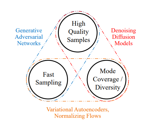
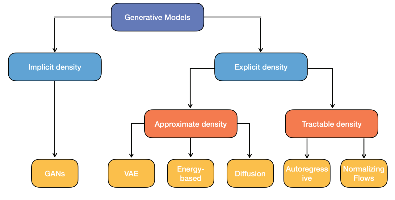
Generative Adversarial Networks: Create images from known noise distribution . 2-player game: generator vs. discriminator (deep NNs). steps gradient descent for steps
- → distinguishes real () vs. generated images
- → creates realistic images
- Objective:
- Theoretical solution: optimum when with value
→ Conditional GAN (CGAN): additional information (e.g. class labels)
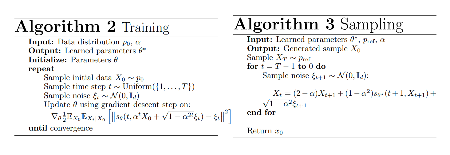
Diffusion models: forward decomposition → add noise, backward decomposition → undo noise Use ancestral sampling starting from a pure Gaussian noise and denoising using Markov chain. Often use U-net architecture (with exponential moving average to stabilise training) with ResNet blocks and self-attention layers. To add additional information (conditional training), the probabilities of neural net should be conditional on .